The elegance of Policy Gradient in reinforcement learning
by Kha Vo
Introduction
In this post, I will present some interesting and somewhat “magical” (at least, to me :-) ) stuffs about Reinforcement Learning (RL), via some simple scenarios. By the end of this post, I hope you will also be thrilled by the capability of what RL can bring. In detail, you will understand:
- How to define the environment to make the agents learn what we want
- The magic of the stochastic policy
- How to code everything in Python, from scratch!
This is the first part of a planned 3 parts I want to write about RL. These posts are for everybody even one with not much prior knowledge in RL, to understand the great power of the stochasticity property of the behaviour of the learned agents.
The Environment
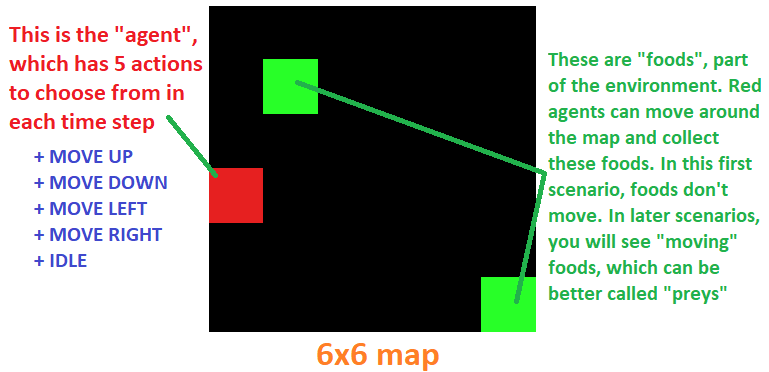
In this first scenario demonstration, I put 1 agent and 2 foods on random positions of the map. Since the agent can move in 4 directions at any time step, they can theoretically reach any cell in this 6x6 map, or any cell in a much much bigger map, say, 1 billion x 1 billion. That means they can theoretically collect as many foods as possible, on an extremely big map.
Turning back on this tiny 6x6 world, I introduce the term “state”, or “observation” of the agent, that is the 3x3 square with the agent in the center. That is equivalent to saying that at any time step, the agent knows (and only knows) the nearest 9 cells surrounding it. Numerically, I can represent each blank cell (no food) as 0, the food-occupied cell as 1, and the wall cells as -1. Indeed, each cell type can be represented by any arbitrary number, because no matter what our model can still automatically adjust this change during training. But it’s better to keep things as simple as possible for the sake of our model training task later on. By the way, these environment objects’ representation makes sense, since food cell (1) is more encouraged to reach, blank cell (0) is uncertain, and wall cell (-1) is encouraged to avoid . By the environment’s definition the agent will stay as-is if it moves directly into the wall.

The Reward
Now the next question is to define a reward function for our agent to learn. This is IMHO the most important thing in developing an RL scenario. We have lots of ways to assign a scalar reward to the agent at each time step, such as
- Reward System 1: At each time step \(t\), if the agent collects food then \(r_t = +1\); if collides with wall then \(r_t = -1\); otherwise \(r_t = 0\).
- Reward System 2: If seeing food around (in the 3x3 local observation) then \(r_t = +1\), if collects food then \(r = +2\), else \(r = -1\). As you can see, both reward systems seem to be correct, because they both encourage the agent to strive for food.
But, sadly, they are all WRONG!! Why?
That’s because we have violated the most basic rule in RL: “We need to tell the agent WHAT to achieve, NOT HOW to achieve”. This is so far the most important quote I extract from the popular textbook “Reinforcement Learning: An Introduction 2nd Edition” of R. Sutton and A. Barto. The main reason is that, if we tell the agent HOW to achieve the goal, it will mostly only attempt to directly optimize the way to achieve the ultimate goal, not the ultimate goal, leading to sub-optimal behavior. As an example, if our goal is to “collect all food in the map”, and we define the reward system as presented above, the agent cannot reach the food if the food is too far from it. The agent’s local observation at each time step is limited (in this case: only 3x3 cells surrounding it), then what if there’s no food around it? It will probably move randomly and desparately looking for food! In other words, the agent is completely blind about the whole world.
Okay. At this point, you may wonder if the agent has only limited local observation, how can it sweep through the whole map looking for food? Is it possible to do so? And how?
Well, that is what I want to show in this post: The Magic!
Stochastic Policy: Make the Blind Bright
Before plunging into the magic, let us first find a way to define a correct reward system first. So far as I said, we need to tell the agent WHAT to achieve, not HOW to achieve. So what should we tell the agent to do in this food-searching scenario? The answer is unimaginarily simple: we define as “win” or “lose” if the agent can get all food or not (after a maximum time). In detail, the reward system is shown as below
- The Correct Reward System:
r = 0for every time step except the final time step;r = +1if no food remains in the last time step;r = -1if there is still food remain in the last time step.
This reward system is like winning or losing the game. In this scenario, I specify the last_time_step = 20. So far this reward formulation matches the concept of “telling the agent WHAT to achieve”, because we only care about the final result. As a result I will describe the game rule once again with this reward system:
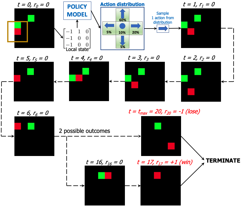
- At \(t = 0\): game starts, place 1 agent and 2 foods randomly on the map.
- At each incremental time step \(t = 1, 2, \dots, 19\), the agent makes a move based on its policy. The reward for each of these time steps is always \(r_t = 0\) because the agent is yet to know it wins or loses the game.
- If at any time step \(t = k\) whenever there is no food remaining, or equivalently saying that the agent just collects the last food at \(t = k \), then assign \(r_k = +1 \) and terminate the game.
- At \(t = 20\): game ends. If all food collected \(r_{20} = +1\), otherwise \(r_{20} = -1\).
In the first glance, this reward system seems to be impossible for the agent to learn, doesn’t it? No, it’s not, because we have a secret magical weapon: Policy Gradient (well, this secret has been revealed for tens of years).
Talking a little bit more about this kind of rewarding system, it is similar to what Google’s Deepmind did when they designed their rewarding system in AlphaZero to master Go game (refer to paper “Mastering the game of Go with deep neural networks and tree search”). Although not exactly the same in this scenario, their rewarding system also only cares about the final outcome of the game: win or lose, and the intermediate states (position of pieces on the board) serve as input observation for the policy model.
Long-term Reward Formulation
Please forgive me for halting to reveal the secret once more. I think at this stage, you might be thinking that: what’s the purpose of all zero-valued rewards at intermediate steps? Are all the actions in those steps meaningless? Indeed, in this particular win-lose formulation, all intermediate steps matter. Imagine if the agent is at the top left corner searching for food at the bottom right corner, then the agent must develop a strategy to feasibly get to the bottom right corner. As a result, all intermediate steps do matter, even so much.
That’s the reason why in RL, the term “long-term reward” is of great importance: it embeds long-term goal into the instantaneous reward samples:
\( R_t = \sum_{k=t}^{t_{\text{max}}} \gamma ^ {k-t} r_t \)
That’s the reason why in RL, the term “long-term reward” is of great importance: it embeds long-term goal into the instantaneous reward samples
Long-term reward can have two variants: average long-term reward (\(\gamma = 1 \)), or discounted long-term reward (\(0 < \gamma < 1 \)). The discount factor \(\gamma \) weighs the importance of future prospect, with a popular chosen value such as \(\gamma = 0.99 \). As a result, we just simply convert each instantaneous reward sample \( r_t \) to its long-term version \( R_t \). Here is an example from the above scenario setting:
- \( r_0 = 0, r_1 = 0, r_2 = 0, \dots, r_{18} = 0, r_{19} = 0, r_{20} = -1 \) which can be converted to
- \( R_0 = -0.818\), \(R_1 = -0.826\), \(R_2 = -0.835\), \(\dots\), \(R_{18} = -0.980\), \(R_{19} = -0.990\) , \(R_{20} = -1.000 \)
Intuitively, because the final outcome is lose (-1), it governs all previous steps, guiding the model learning process that “each of the action in those steps will lead to a bad result”, where sooner steps have less influence. One can argue that, what if from step 1 to step 10 the agent luckily randomly get all correct decisions, but from step 11 to step 20 it produces bad decisions, how can we know? And is it right thing to do when telling the model that all steps are bad just because the final result is bad? The answer is that case can possibly happen, but in a long session of training where all combinations of sequences of actions can be swept through, on average we would expect correct actions lead to good outcome. To understand more about this interesting fact (indeed, it is the magic of Policy Gradient), I suggest the reader to this great article about Policy Gradient written by a well-known machine-learning Stanford guy named Andrej Karpathy.
Finally the Magic: Policy Gradient Let us see a trained agent using PG on a 6x6 map:
Not much interesting, is it? Wait, am I the only one seeing a strange behaviour of the agent? Is it following the wall counter-clockwise? And why?
As you already know at each time step the agent can only observe 9 nearest cells (which I call the “view”) surrounding it. Then, in this small environment the agent must find a way to exploit all information from the state space (equivalent to different views) to develop a strategy to collect as many food in the shortest time as possible. To understand more about the whole behaviour in the global concept, here I show the trained behaviour with respect to some typical different agent views, and give some explanation on it:

- The bottom-right subfigure presents the probability distribution of all 5 possible actions given the input view of the agent next to the bottom-side wall with no food around. The trained agent prefers to go right. The similar behaviours are seen if the agent is next to the left-hand wall (it prefers to down) or right-hand wall (it prefers to go up), which I do not show here.
- The bottom-left subfigure demonstrates that whenever a food presents in the view, the agent will most likely to move itself to the food. This behaviour is also seen in other views with the presence of food.
- Both top subfigures are key to explain the agent behaviour intuitively. As I trained the agent in a 6x6 grid-world, if it always follows the wall consistently, there’s no way to reach the foods at the center cells of the map. So from learning the agent must find itself a way to avoid this. Now let us carefully see the agent’s behaviour again in the animation, you can notice that it does not strictly follow the top wall. Instead, it tends to turn down a little bit more when it is adjacent to the top wall. This behaviour is encouraging the agent to explore the world more, although whenever in the completely blind state (nothing around), it must however follows a strict trained strategy to optimise the ultimate goal that has been given for learning. The top-left subfigure suggests that the agent prefers to go right and down. That is the result in accompany with all other states’ behavious to optimise the goal: since the agent already strictly follows the left, right, and bottom walls, it must not strictly follows the top wall because if so (as we, human, can easily understand) it can’t reach center food cells. So, the behaviour in this completely black view is the optimal when taking all other views’ behaviours into account.
For clearer understanding, let’s have a look at the probability of each cell of being stamped on by the agent. The below figure was retrieved by letting the trained agent move 10,000 steps, then counting the number of times each cell is met. The numbers on the plot are the percentage (in %) of that cell being met.
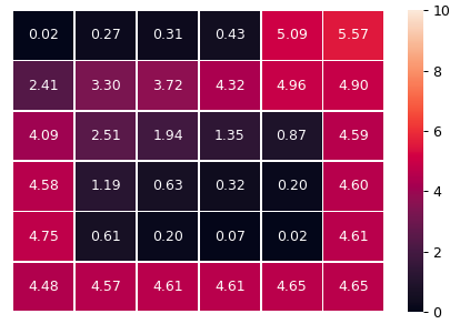
Some cells are rarely met with extremely low frequency, such as the top left cell (0.02%). That is not a problem if a food is placed there, because whenever the agent falls in the cell below it, which has high probability (2.41%), the agent will discover the food and move towards it easily. This heatmap plot, in conclusion, confirms that the agent has positively chance to reach all foods in the 6x6 map.
Now one question arises: how do it behave if being thrown into a bigger world, say, 15x15? Here is the result
.gif)
As shown, with the same policy trained in the 6x6 world, the agent cannot reach some middle cells in the 15x15 world. Let us have a look at the heatmap in the 15x15 world too
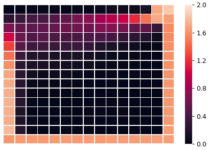
Not surprisingly there are a lot of cells which the agent cannot reach, resulting in remaining foods in some particular cells that the agent can never see.
So, what if we train the agent in the 15x15 world? How will it fare with this big world?
Let’s see the result of the agent trained in the 15x15 world
Voila! Although still struggling and time-consuming to see all cells, the agent can still explore the whole map by a better policy when trained in this bigger world. One more interesting fact is that now it moves clockwise instead of counter-clockwise. Since clockwise and counter-clockwise behaviours are nothing different from the global perspective, the policy can reach and converge to either of them first (by luck, of course) when training.
Conclusion
-
From just the local view, the agent can achieve a good policy (behaviour) that can optimise the global ultimate goal, by exploiting all information it can collectively collect from the environment during training. In other words, this “blind” agent becomes bright about the whole world after training. What if we insert some marks in the map, such as an oak tree at cell (4,5) and 2 palm trees at cell (12, 13) and (4, 9)? The answer is that the agent will exploit them very well, resulting in better behaviour than without them.
-
The magic of the trained policy is based on the Policy Gradient theorem, which allows the optimal behaviour to be stochastic. In other words, the agent can still pick a sub-optimal action in a specific state to encourage exploration with guidance. The stochasticicy of the behaviour allows the resulting trained action probability distributions of different states to collaborate with each other, without violating the stationarity Markov assumption of the environment. For easy understanding, relate this mechanism to chess games: to win a game (check-mate state) one must reach the previous chess board state which has high probability of check-mating the opponent. Then to reach that prenultimate state one has to reach the state before that.
-
What if we train multiple agents, say, 2 agents, in the 15x15 world? The agents will see each other if they are near, then we have a sense of collaboration here. But training 2 agents in the same time requires many more technical considerations. Will the 2 collaborated agents fare better than the 2 single-trained agents on the map?
That will be the main treat in Part 2. Stay tuned, and thanks for reading!
Wait! Are you waiting for the code? Okay, almost forget, but I’m still here. I’d prepared a python notebook here which includes all above experiments. The amazing thing is that this code does not require any Reinforcement-Learning-specific dependencies, and not require GPU too! You can try to train with your local CPU in 20 minutes to achieve those presented result, and animate it! Code for Magic of Reinforcement Learning - Part 1
Gentle Reminder: Please feel free to re-use the materials here with citing required, by just simply copy the article source link, or my name. So much thanks for your kindness.